Overview

Problem Statement

The basic scope of the project is that given a Spotify playlist, to build a regression model to predict the success of the playlist measured by the potential number of followers. With this model, we can generate a high-quality playlist, given a specified genre and a pool of tracks to choose from.

To achieve the task of predicting followers, we can train a regression model on a set of labelled training data, with explanatory variables being a set of features derived from the playlist and its tracks, and response variable being the follower of the playlist. To generate a playlist, we will first take in inputs from the user, and then use our followers prediction model to identify the playlist that is predicted to have the most followers.

Data Description

We chose 24 most popular genres from in Spotify, and collected information of top 50 playlist results with Spotify API. For each playlist, we collected the features of its basic information (e.g., number of followers), and also obtained a list of tracks (i.e., songs) within the playlist. Finally, we sent another query to collect audio features for each track.

With Spotify API, we collected and stored three data sets in JSON format, they are genres_playlists (genres and corresponding playlists), playlists_tracks (playlists and corresponding tracks) and tracks_features (tracks and corresponding features). We merged three dataset into a single data frame with the combination of being the unique identifier of an observation.

Table 1. All variables in the combined data frame
Variable Name	Type	Description
acousticness	Quantitative, float	Sound through acoustic, as opposed to electric
danceability	Quantitative, float	Dance friendly measurement
duration_ms	Quantitative, float	Total length of music in second
energy	Quantitative, float	Identify the different pitches and frequencies, and create high- and low-pitch sound waves
instrumentalness	Quantitative, float	The variety of instruments appeared
key	Categorical, int	Scale of music, a set of sharp (♯), flat (♭)
liveness	Quantitative, float	Dynamically performed assertion of human presence within a technological network of communication
loudness	Quantitative, float	Sound pressure
mode	Categorical, int	Descending diatonic scales in the music of classical Greece
speechiness	Quantitative, float	measures the number of spoken words
tempo	Categorical, int	timing of music, or the speed
time_signature	Categorical, int	Beats (pulses) contained in each measure (bar)
valence	Quantitative, float	intrinsic attractiveness or aversiveness of an event, object, or situation
genre	Categorical, str	Genre of the track
popularity	Quantitative, int	Popularity measurement, range from 1 to 100
followers	Quantitative, int	Number of followers

Challenges

There are several challenges we are faced with. First, the data is not ready-to-use. We need to collect our own data through Spotify Web API. It is up to us how we want to organize our data. Second, the data has relatively limited predictors considering the difficulty of the prediction task. These predictors are mostly at track-level, so we need to aggregate them effectively into a playlist-level in order to perform regression analysis. Another challenge lies in the playlist generation process. Searching for the playlist that is predicted to have the highest followers is an expensive combinatorial problem. We need to find alternatives to brute-force search.

Exploratory Data Analysis

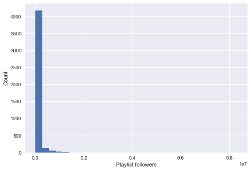
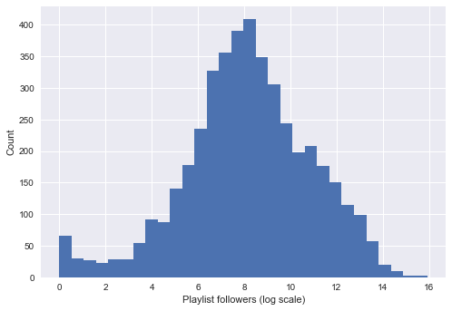
Distribution of predictors and number of followers

We generated a barplot of the average values of different audio features for different genres. In order for the plot to be more informative, we normalized the range of each feature to be (0, 1). The main idea between this visualization is to show that different genres have different profiles of audio features, which determined their uniqueness.

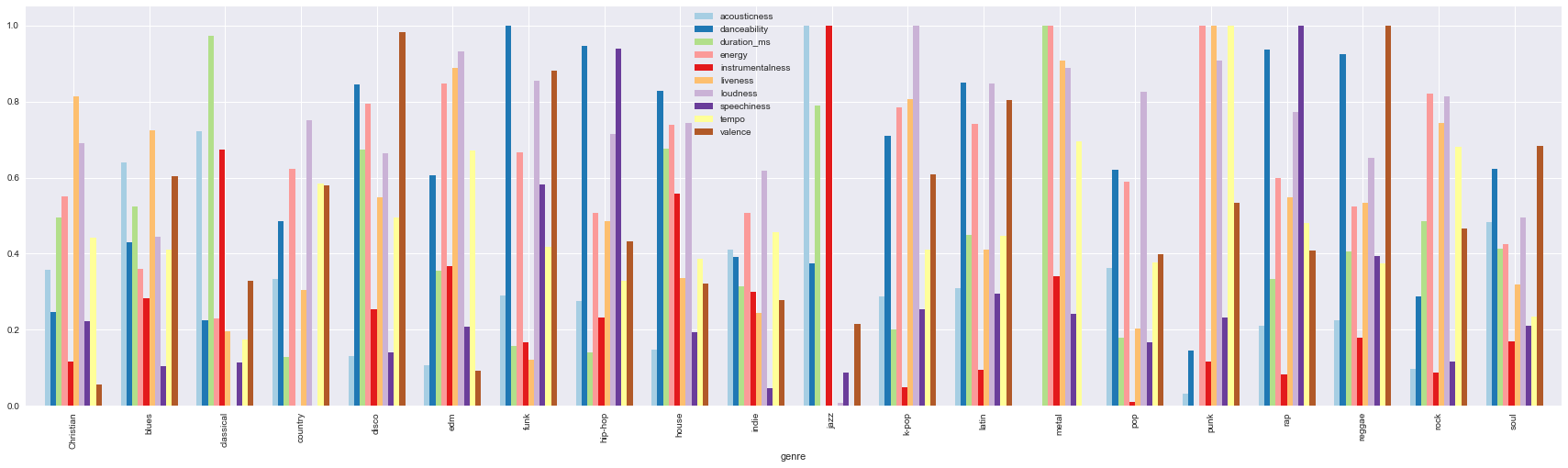
Figure 1. Average values of audio features for different genres

For example, funk music has high danceability, jazz music has high instrumentalness, hip-hop has high speechiness, etc. This tells us these audio features can be very distinguishing. We also want to understand the distribution of the response variable - number of followers for each playlist. Thus, we plotted a set of boxplots of followers for each genre. In general, pop, hip-hop, classical and rock have relatively higher median and variance.

We also want to understand the distribution of the response variable - number of followers for each playlist. Thus, we plotted a set of boxplots of followers for each genre. In general, pop, hip-hop, classical and rock have relatively higher median and variance.

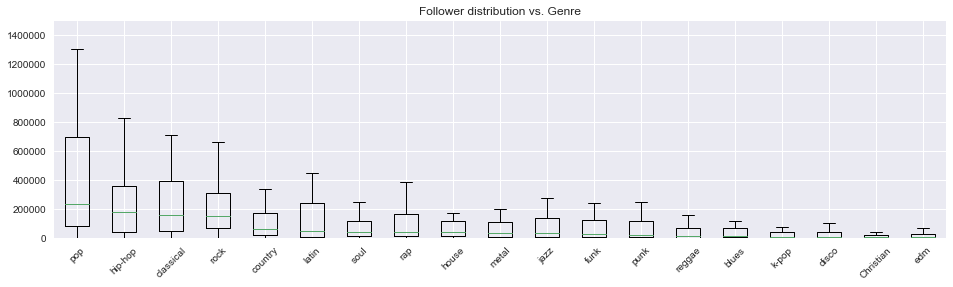
Figure 2. Distribution of number of followers for different genres

Relationship between predictors and number of followers

With an aim to identify useful predictors for building regression models, we plotted scatter plot of the number of followers with respect to different predictors. Here possible predictors include audio features of the tracks within the playlist, and the popularity of them (measured by how much it has been played on Spotify). However, as each song in a playlist can have a set of values, we will need some method of aggregation to construct playlist-level features. Here, we explored two ways, using mean to capture overall level, and using standard deviation to capture diversity within the playlist. In order to show clearer relationships, the graphs below might exclude some outliers that affect the visual.

When using mean as the aggregation method, we observe that some audio features, such as loudness and popularity (Fig 3), positively contribute to the number of followers. We also observed that instrumentalness is negatively correlated with number of followers. For tempo, it seems to have an interval that correlates more to high number of followers. This calls for feature engineering in subsequent steps, such as discretization of the tempo variable.

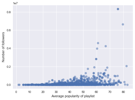
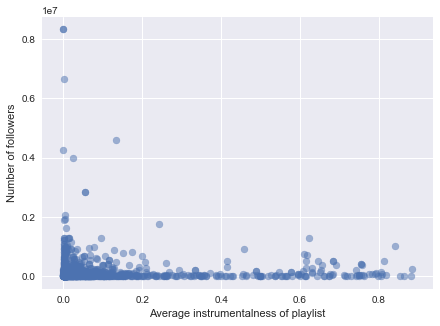
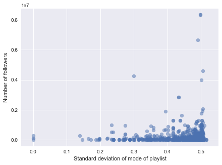
Figure 3. Scatterplots of number of followers against predictors. (left: average popularity, middle: average instrumentalness, right: standard deviation of mode)

When using standard deviation, we can capture whether feature diversity in a playlist has relationship with the playlist follower numbers. So if we observe skewness in the plot, it means that either diversity of homogeneity is favorable to gaining higher followers. We observe that when a playlist has diversity in mode is positively correlated with the number of followers. This makes sense as mode directly determines the mode of the song. A relatively large diversity of tempo also seems to give rise to high followers, as the distribution is right-skewed.

Relationship between predictors and number of followers for different genres

As in the end we need to generate playlist for a specified genre, the model should be able to adapt to different genres. Therefore, we want to explore that for playlist in different genres, whether there is interaction between genres and the predictors’ correlation with the number of followers. Thus, we created a heatmap shown below. Each cell represents the correlation between predictors (represented by vertical axis) in a particular genre (represented by horizontal axis) and the number of followers of the playlist.

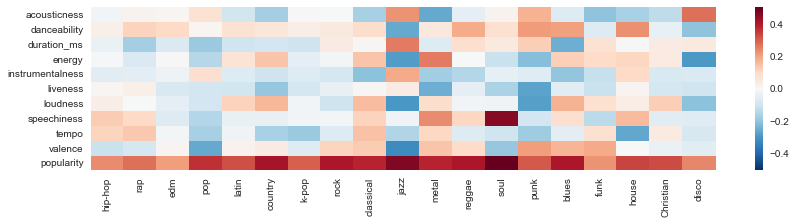
Figure 4. Heatmap of correlation of predictors with number of followers by genres

There is plenty of information in the heatmap. To name a few, popularity has positive correlation with followers across genres; speechiness is positively correlated with followers in soul music; valence is negatively correlated with followers in pop music; the correlation for different features is more bipolar in jazz, etc. This allows us to create interactions in the regression model to predict number of followers.

Followers Prediction

Data Transformation

When we explore the distribution of the response variable, we found out that the distribution of playlist followers is heavily right-skewed. After transforming it to its logarithm scale, the distribution becomes much more normal. Therefore, in all our following modeling practices, we adopted the log scale of the original response variable.

Figure 5. Histogram of playlist followers, before and after log transformation

Baseline Model

As a first step, we want to have an initial model that uses the most basic features to benchmark against.

Table 1. Baseline model information
Model	Linear Regression
Preprocessing	None
Feature	Mean audio features, mean popularity
Training R Squared	0.0670
Testing R Squared	0.0491

Feature Engineering

We went through multiple iterations of feature engineering, with an aim to extract more useful information from the collected data.

One-hot encoding of categorical features. In the audio features, key and time_signature are all categorical variables that do not have any ordinal relationships. Therefore, they require one-hot encoding to prevent them to be interpreted as continuous variables by our regression model. From the heatmap in our EDA, we also know that some of the genre might have a significant correlation with number of followers, and thus should also be taken into account as our feature in the model.
Top singers count. As a continuation of the maximum track popularity feature, we find that people sometimes are likely to follow a playlist if the playlist contains the artists/singers they like. We think that the number of followers of a playlist could have a high correlation with the number of top artists/singers in that playlist. Therefore we want to build a new predictor that measure how many songs in the playlist falls under this category. For this new feature we scraped the Billboard website to get the 100 most popular artists and also matched the names of these artists with the artist id from Spotify. Based on this list, we computed how many songs in the playlist belong to the 100 artists.
Maximum track popularity. Based on our original Spotify experience, it is very common that people sometimes follow a specific playlist through a particular song they are looking for. It is also very common that certain playlists were recommended to users by Spotify's recommendation system because users listen to the most popular song in that playlist. Therefore, it is very likely that the most popular track in a playlist will affect the popularity of this playlist.
Number of tracks, artists and albums. Playlist serves an important purpose of broadening one's horizon of songs. Therefore, a playlist's diversity, measured by the number of albums and artists, could potentially affect its followers. Playlists with larger number of albums and artists are potentially more popular. For example, a playlist that is dominated by 2 or 3 popular singers might be less valuable than a playlist that has songs from a wide range of artists. The same applies to albums. For number of tracks, this is even a more important indicator of the richness and diversity of a playlist.
Standard deviations of audio features. From our EDA, we reckoned that sometimes aggregation methods other than mean could also contain useful information about a playlist. For example, a playlist that has high standard deviation in mode might lead to higher diversity in mood.

With each new addition, we recorded its corresponding effect in model performance. These models are still built with linear regression.

Table 2. Training and testing R squared as a result of new features
#	New Feature	Training R Squared	Testing R Squared
0	-	0.0670	0.0491
1	One-hot encoding of categorical features	0.4705	0.4494
2	Top singers count	0.4767	0.4588
3	Maximum track popularity	0.4788	0.4616
4	Number of tracks, artists and albums	0.5012	0.4953
5	Standard deviations of audio features	0.5107	0.5098

Figure 6. Evolution of R Squared during feature engineering

As a last step of feature engineering, we added in the interaction terms between genre and all other predictors. This is motivated by our EDA that for different genres, different predictors might have particularly high or low effect than they normally do. Although train test R Squared 0.68, test set R Squared dropped to below 0.3. This is a clear sign for overfitting. Thus, in the next section, we resort to PCA and feature selection to reduce the dimension of the data matrix.

Dimensionality Reduction

From the attempts above, we realized that although we interaction terms might carry useful trends, adding all of them is subject to heavy overfitting. Hence, we want to explore two different options of dimensionality reduction: PCA and feature selection. After this, we will fit different models to the reduced data matrix, and compare their performance against each other, and also against the best performance before adding interaction terms.

Principal Component Analysis (PCA)

We developed a 5-fold cross validation scheme to select the best n_component for the PCA transformation. We also plotted out the evolution of cross validation training and testing R2 to better visualize the trend of model accuracies. We can see that both R2 increase swiftly as the number of principal components increases from 1 to 21. Since then, R2 only slowly increase with high volatility.

Figure 7. Cross validation training and testing R Squared for different n_components

Now, as the data dimension has been sufficiently reduced, we built various regression models and compared their test set performance.

Figure 8. After PCA: test set R Squared comparison

Forward Feature Selection

Another way to shrink feature space is through forward feature selection. We used linear regression's BIC score as the criterion for choosing features. Below we printed the change in BIC with increasing amount of features in the model.

Figure 9. Evolution of BIC with increasing number of features

We also enumerated the top 10 features that are first selected into the model, many of which are highly interpretable.

Table 3. Top 10 features selected by forward feature selection
Sequence	Feature Name
1	genre_hollywoods x max_popularity
2	genre_k-pop x speechiness
3	genre_opera
4	genre_pop x popularity
5	genre_rock x popularity
6	genre_classical x popularity
7	genre_hip-hop x popularity
8	genre_house x popularity
9	genre_indie x num_artists
10	popularity_std

For example, hollywood playlist depends highly on tracks' popularity; opera playlist might inherent receive lower number of followers; rap music has distinct interaction with average valence of tracks. As expected, we also see many genres have interaction with popularity, given that although popularity is contributive in general, it still has different extent of contribution depending on the genres.

At last, we also compared the test set performance across different regression models.

Figure 10. After forward feature selection: test set R Squared comparison

Feed-Forward Neural Network

After using the approaches above discussed in class, we also implemented a feed forward neural network (FNN). Our FNN used two hidden layers, with linear function between each two layers. After attempting several activation functions of two hidden layers, we found that Tanh on the first hidden layer and sigmoid function on the second hidden layer provides the best performance on the test dataset. Although it did not achieve the best R2 score than the best ensemble models above after feature transformations, it performed much better than most models (e.g., Linear regressor, Elastic Net regression) given the same feature data before dimensionality reduction. Moreover, it fits relatively faster than the best ensemble models such as Random Forest regressor, and saves a huge amount of time of manual feature engineering.

Figure 11. Evolution of testing R Squared with epoch

We fitted the FNN on both the data before and after PCA. The two versions achieve almost identity final test set R Squared. This shows neural network's capability of control overfitting through its hidden layer and choice of activation function.

Playlist Generator

With a followers prediction model in place, what can we do with it? A direct application is to algorithmically generate a playlist out of many track candidates.

The problem comes in when the pool of candidates is too large, which is true for Spotify. Therefore, we will need some track-level filtering to help us narrow down the search space. From our modeling, we understand that popularity is a key influencer of playlist followers. Therefore, we can use tracks' individual popularity as a criterion to do initial filtering of tracks. We adopted a scaling factor of 3 in our analysis, which means for a desired playlist length d, we kept only the top 3d most popular tracks. After this step, we explored two approaches:

Exhaustive search.
We iterate through all combinations of the narrowed-down pool and use our followers prediction model an evaluation function to select the highest-scoring combination.

Greedy search.
In this approach, we start with an empty playlist. At each step, we try different tracks to the existing playlist, and select the track that gives us the most improvement based on our followers prediction model.

In general, our playlist generator has the signature of playlist_generator(library, model, genre, length). Library stands for all the track candidates; model gives the followers prediction model; genre and length specify the genre and length of the playlist to be generated.

Below, we compared the performance of these two approaches plus a baseline defined by random generation. The goal is to achieve high predicted followers for the generated playlist, and also with relatively small computation time. We can see that in our examples, greedy method is able to match the predicted followers of the exhaustive method, but with far smaller computational cost, usually within 2 to 3 seconds. Greedy approach's computational cost also grows linearly, as opposed to exhaustive search's exponential growth.

Figure 12. Comparison of predicted followers for different playlist generation approaches

Figure 13. Comparison of computation time for different playlist generation approaches

Conclusion

In this project, we had a chance to explore the entire process of data analysis: from data crawling, data cleaning, EDA, to building models, tuning models and model selections. Walking through this complete process as a group gave us a better insight in data science. We have met many obstacles throughout the process and we are very glad that we overcame all of them.

When first approaching this project, all we were considering was feature engineering and model designs, we were not too prepared with crawling the data. This actually was gave us many troubles. Subject to the access time limit of Spotify api, the data crawling turned out to be very time consuming. We untimately decided to automate every step of our crawling code and host it on an AWS server to finish the crawling job. The whole crawling script took 48 hours to finish its job and gave us ~350,000 tracks and ~4400 playlists in 24 different genres. The careful design of data crawling actually saved us a lot of time on data cleaning. After merging the dataframes we had, we ended up only dropping several row of data with 'nan' term introduced in the aggregation of our feature engineering step.

After that, we came to EDA as well as feature engineering. We find EDA to be extremely useful to the feature engineering. Most of our features are actually designed with the knowledge of our EDA. For example, we had a large heatmap showing the correlations of audio features and followers in different genres. We found many genres' correlations with number of followers are very sensitive to the changes in audio features. This gave us a very important motivation to design the interaction features between genres and audio features. Also, we found the total number of tracks in a playlist has a very high correlation with followers. This also turned out to be a very powerful feature as we reported previously in the notebook. We also made use of alternative data sources to contruct new features. Specifically, we scraped the Billboard top 100 singers to include top singers count as a predictor, which also helped the model to some extent. As we shown in the notebook, every new feature we introduced to the model resulted in an increase in the R Squared score.

To combat the overfitting caused by adding interaction terms, we adopted PCA and forward feature selection to reduce the dimensionality of our model. Then, we came down to fitting, selecting and tuning models. In this part we exaustively tried every model we have learnt in class, as well as some extra models we did not have exposure in the class yet. Specifically, we implemented a feed-forward Neural Network with 2 hidden layers in PyTorch, and employed Extra Trees and Extreme Gradient Boosting as extra models. We also collected the best-performing models we found and stacked them together to form a meta model, which usually gave us the best performance. In a nutshell, both PCA and feature selection, coupled with a carefully tuned model, were able to achieve a test set R Squared of over 0.57, a significant improvement on the model without interaction terms and dimensionality reduction. The advantage of feature selection over PCA is that, the selected features and the order they are selected give us extra information about their importance to the model.

In the end, the best model without interaction terms achieved a test set R Squared of 0.5098, and the best model with interaction terms achieved a test set R Squared of 0.5702. However, the sacrifice is more data processing steps (adding interaction terms, dimensionality reduction), and a more complicated model. In terms of model choices, tree based models generally perform better than other models. This might be due to tree based models' capability to capture non-linear relationships between predictors and response variables.

Lastly, we made use of our followers prediction model to build a playlist generator. We attempted three different approaches of narrowing down the search space, random, exhaustive and greedy. We compared their performance in terms of predicted followers and computational cost, and arrived at a conclusion that with a significant reduction in computation time, greedy search is able to generate playlists almost as high quality as that of exhaustive search. Thus, it might be the more viable approach among the three.

Future Work

With regard to the followers prediction model, it can potentially benefit from having more useful features. For example, the model can include features that capture the credibility of the playlist's creator. If the creator has published many other popular playlists in the past, his/her future playlist is more likely to receive a high number of followers.

For the playlist generator, we could potentially further extend the greedy method to avoid reevaluating all the options at each iteration. One option is to keep track of the best-scoring tracks and only evaluate these tracks at the next iteration. Another option is to incorporate similarity between tracks as an additional criterion of generating playlist.

If we could gather user-specific information, we could personalize this playlist recommendation system to cater to users' taste of music. This system can even be integrated into Spotify's current system to allow for a more thoughtful user experience.

Related Works and References

Kaggle has a similar project called Audio Features for Playlist Creation. Instead of a regression model to predict the number of followers, the project is to classify classify songs into themes such as dinner, sleep, party or workout. We referred to some kernels in the project to get inspiration on feature engineering.

To obtain data regarding genres, playlists and tracks on Spotify, we used Spotify's Web API. This page provided the most help regarding the various get requests that are allowed on the API.

We referred to PyTorch's documentation to develop our feed-forward neural network.